Exemplary Usage

In this documentation, exemplary use cases for the Gabor wavelet transform (and related) classes are detailed.

Gabor wavelets

The bob.ip.gabor.Wavelet class can be used to create Gabor wavelets. The parametrization is according to what is explained in detail in [Guenther2011].

The Gabor wavelets by default are in frequency domain. To create a Gabor wavelet of size (128, 128) with the vertical orientation and frequency , you call:

>>> wavelet = bob.ip.gabor.Wavelet(resolution = (128, 128), frequency = (math.pi/2, 0))

To compute the wavelet transform, an image of the same resolution in frequency domain must be present:

>>> test_image = numpy.zeros((128,128), numpy.uint8)
>>> test_image[32:96, 32:96] = 255
>>> freq_image = bob.sp.fft(test_image.astype(numpy.complex128))

Now, the wavelet transform with the given wavelet can be applied:

>>> transformed_freq_image = wavelet.transform(freq_image)

To get the transformed image in spatial domain, it needs to be transformed back using bob.sp.ifft:

>>> transformed_image = bob.sp.ifft(transformed_freq_image)

Please note that the resulting image is complex valued. You can look at its real and its absolute components:

>>> real_image = numpy.real(transformed_image)
>>> abs_image = numpy.abs(transformed_image)

A full working example (including the plotting) is given below:

import numpy
import math
import bob.ip.gabor
import bob.sp

# create exemplary image
image = numpy.zeros((128,128), numpy.uint8)
image[32:96,32:96] = 255

# create Gabor wavelet
wavelet = bob.ip.gabor.Wavelet(resolution = (128, 128), frequency = (math.pi/8., 0))

# compute wavelet transform in frequency domain
freq_image = bob.sp.fft(image.astype(numpy.complex128))
transformed_freq_image = wavelet.transform(freq_image)
transformed_image = bob.sp.ifft(transformed_freq_image)

# get layers of the image
real_image = numpy.real(transformed_image)
abs_image = numpy.abs(transformed_image)

# get the wavelet in spatial domain
spat_wavelet = bob.sp.ifft(wavelet.wavelet.astype(numpy.complex128))
real_wavelet = numpy.real(spat_wavelet)
# align wavelet to show it centered
aligned_wavelet = numpy.roll(numpy.roll(real_wavelet, 64, 0), 64, 1)

# create figure
from matplotlib import pyplot
pyplot.figure(figsize=(20,5))
pyplot.subplot(141)
pyplot.imshow(image, cmap='gray')
pyplot.title("Original image")

pyplot.subplot(142)
pyplot.imshow(aligned_wavelet, cmap='gray')
pyplot.title("Gabor wavelet")

pyplot.subplot(143)
pyplot.imshow(real_image, cmap='gray')
pyplot.title("Real part")

pyplot.subplot(144)
pyplot.imshow(abs_image, cmap='gray')
pyplot.title("Abs part")

pyplot.show()

(Source code, png, hires.png, pdf)

Gabor wavelet transform

The bob.ip.gabor.Transform class is performs a Gabor wavelet transform using a discrete family of Gabor wavelets. The family of Gabor wavelets is composed of wavelets in different scales and orientations. By default, the family consists of Gabor wavelets in 5 scales and 8 orientations:

>>> gwt = bob.ip.gabor.Transform()
>>> gwt.number_of_scales
5
>>> gwt.number_of_directions
8
>>> gwt.number_of_wavelets
40

When transforming an image, all Gabor wavelets will be applied to it. In opposition to the bob.ip.gabor.Wavelet class (see above), the parameters to the bob.ip.gabor.Transform expects all input and output images to be in spatial domain:

>>> trafo_image = gwt.transform(test_image)
>>> trafo_image.shape
(40, 128, 128)
>>> trafo_image.dtype
dtype('complex128')

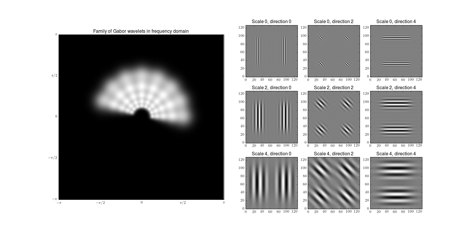
The result is a 40 layer image that contains the complex-valued results of the transform. A few of these results (together with the according wavelets) can be seen here:

import numpy
import math
import bob.ip.gabor
import bob.sp

# create test image
image = numpy.zeros((128,128), numpy.float)
image[32:96,32:96] = 255

# compute the Gabor wavelet transform
gwt = bob.ip.gabor.Transform()
trafo_image = gwt(image)

# create image representation of all Gabor wavelets in frequency domain
wavelets_image = numpy.zeros((128,128), numpy.float)

# compute the sum over all wavelets
for wavelet in gwt.wavelets:
  wavelets_image += wavelet.wavelet

# align the wavelets so that the center is in the image center
aligned_wavelets_image = numpy.roll(numpy.roll(wavelets_image, 64, 0), 64, 1)

# create figure
import matplotlib
matplotlib.rc('text', usetex=True)
# plot wavelets image
from matplotlib import pyplot
pyplot.figure(figsize=(20,10))
pyplot.subplot(121)
pyplot.imshow(aligned_wavelets_image, cmap='gray')
pyplot.title("Family of Gabor wavelets in frequency domain")
pyplot.xticks((0, 32, 64, 96, 128), ("$-\pi$", "$-\pi/2$", "$0$", "$\pi/2$", "$\pi$"))
pyplot.yticks((0, 32, 64, 96, 128), ("$-\pi$", "$-\pi/2$", "$0$", "$\pi/2$", "$\pi$"))
pyplot.gca().invert_yaxis()

# plot the results of the transform for some wavelets
for scale in (0,2,4):
  for direction in (0,2,4):
    pyplot.subplot(3,6,4+scale*3+direction/2)
    pyplot.imshow(numpy.real(trafo_image[scale*gwt.number_of_directions+direction]), cmap='gray')
    pyplot.title("Scale %d, direction %d" % (scale, direction))
    pyplot.gca().invert_yaxis()

pyplot.show()

(Source code, png, hires.png, pdf)

The first row displays the Gabor wavelet family in frequency domain can be obtained by (cf. Figure 2.2 of [Guenther2011]).

Gabor jet and their similarities

A Gabor jet is the collection of the (complex valued) responses of all Gabor wavelets of the family at a certain point in the image. The Gabor jet is a local texture descriptor, that can be used for various applications. To extract the texture from the right eye landmark from a facial image, one can simply call:

>>> image = bob.ip.color.rgb_to_gray(bob.io.base.load(bob.io.base.test_utils.datafile("testimage.jpg", 'bob.ip.gabor')))
>>> gwt = bob.ip.gabor.Transform()
>>> trafo_image = gwt(image)
>>> eye_jet = bob.ip.gabor.Jet(trafo_image, (177, 131))
>>> eye_jet.length
40

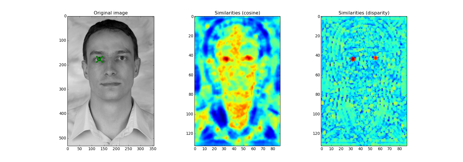
One of these applications is to locate the texture in a given image. E.g., one might locate the position of the eye by scanning over the whole image. At each position in the image, the similarity between the reference Gabor jet and the Gabor jet at this location is computed. For this computation, both traditional [Wiskott1997] and innovative [Guenther2012] similarity functions can be used. In fact, since the texture descriptor is stable against small shifts, only every 4th pixel will be extracted, and the original offset position is not included:

import numpy
import bob.io.base
import bob.io.image
import bob.io.base.test_utils
import bob.ip.color
import bob.ip.gabor

# load test image
image = bob.ip.color.rgb_to_gray(bob.io.base.load(bob.io.base.test_utils.datafile("testimage.jpg", 'bob.ip.gabor')))
# perform Gabor wavelet transform on image
gwt = bob.ip.gabor.Transform()
trafo_image = gwt(image)
# extract Gabor jet at right eye location
pos = (177, 131)
eye_jet = bob.ip.gabor.Jet(trafo_image, pos)

print (image.shape)
# compute similarity field over the whole image
cos_sim = bob.ip.gabor.Similarity("ScalarProduct")
disp_sim = bob.ip.gabor.Similarity("Disparity", gwt)
cos_image = numpy.zeros(((image.shape[0]+1)//4, (image.shape[1]+1)//4))
disp_image = numpy.zeros(((image.shape[0]+1)//4, (image.shape[1]+1)//4))
# .. re-use the same Gabor jet object to avoid memory allocation
image_jet = bob.ip.gabor.Jet()
for y in range(2, image.shape[0], 4):
  for x in range(2, image.shape[1], 4):
    image_jet.extract(trafo_image, (y,x))
    cos_image[y//4,x//4] = cos_sim(image_jet, eye_jet)
    disp_image[y//4,x//4] = disp_sim(image_jet, eye_jet)

# plot the image and the similarity map side-by-side
from matplotlib import pyplot
pyplot.figure(figsize=(20,7))
pyplot.subplot(131)
pyplot.imshow(image, cmap='gray')
pyplot.plot(pos[1], pos[0], "gx", markersize=20, mew=4)
pyplot.axis([0, image.shape[1], image.shape[0], 0])
#pyplot.axis("scaled")
pyplot.title("Original image")

pyplot.subplot(132)
pyplot.imshow(cos_image, cmap='jet')
pyplot.title("Similarities (cosine)")

pyplot.subplot(133)
pyplot.imshow(disp_image, cmap='jet')
pyplot.title("Similarities (disparity)")

pyplot.show()

(Source code, png, hires.png, pdf)

As can be clearly seen, both eye regions have high similarities with both similarity functions (remember, we are searching with only the right eye Gabor jet). The difference is in the other regions of the face. While the traditional cosine similarity (aka. 'ScalarProduct') has high similarity values all over the image, the novel 'Disparity' similarity highlights specifically the eye regions.

The disparity similarity function has even another use case. It can estimate the disparity (difference in spatial position) between two Gabor jets, as long as they stem from a similar region:

>>> disp_sim = bob.ip.gabor.Similarity("Disparity", gwt)
>>> pos = (231, 173)
>>> dist = (5, 6)
>>> jet1 = bob.ip.gabor.Jet(trafo_image, pos)
>>> jet2 = bob.ip.gabor.Jet(trafo_image, (pos[0] - dist[0], pos[1] - dist[1]))
>>> print ("%1.3f, %1.3f" % tuple(disp_sim.disparity(jet1, jet2)))
4.816, 5.683

In this small example we have used Gabor jets from the same image to compute the disparity. However, it has also been shown in [Guenther2011] that also a Gabor jet from one image can be found in another image, even of a different person. Hence, this function can be used to localize landmarks.

Note

The area, where useful disparities can be computed, can be increased by using a different parametrization of the Gabor wavelet transform, e.g., by increasing the number_of_scales in the bob.ip.gabor.Transform constructor.

Gabor graphs

Finally, graphs of Gabor jets can be used to identify a person. The bob.ip.gabor.Graph class is designed to extract Gabor jets at regular grid positions in the image. Particularly for face recognition, the grid graph can be aligned to eye positions, but also a regular grid can be created by specifying the first and the last node, as well as the step width:

>>> graph = bob.ip.gabor.Graph(first=(100,100), last=(image.shape[0]-100, image.shape[1]-100), step = (20, 20))
>>> graph.number_of_nodes
136
>>> graph.nodes[0]
(100, 100)
>>> graph.nodes[135]
(420, 240)

This graph can be used to extract Gabor jets from a Gabor transformed image:

>>> jets = graph.extract(trafo_image)
>>> len(jets)
136

When graphs are extracted from two facial images, the average similarity of the Gabor jets can be used to define, whether two images contain the the same identities. A complete example on the AT&T database can be found in the xbob.example.faceverify package.

Todo

Adapt http://pypi.python.org/pypi/xbob.example.faceverify so that it actually uses the bob.ip.gabor package.