Users Guide

As in most modern face detectors, we also apply a cascaded classifier for detecting faces. In this package, we provide a pre-trained classifier for upright frontal faces, but the cascade can be re-trained using own data.

Face Detection

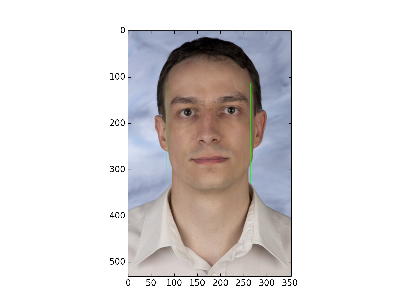
The most simple face detection task is to detect a single face in an image. This task can be achieved using a single command:

>>> face_image = bob.io.base.load('testimage.jpg') 
>>> bounding_box, quality = bob.ip.facedetect.detect_single_face(face_image)
>>> print (quality, bounding_box.topleft, bounding_box.size)
33.1136586165 (113, 84) (216, 180)

(Source code, png, hires.png, pdf)

As you can see, the bounding box is not square as for other face detectors, but has an aspect ratio of 5:6. The function bob.ip.facedetect.detect_single_face() has several optional parameters with proper default values. The first optional parameter specifies the bob.ip.facedetect.Cascade, which contains the classifier cascade. We will see later, how this cascade can be re-trained.

The minimum_overlap parameter defines the minimum overlap that patches of multiple detections of the same face might have. If set to 1 (or None), only the bounding box of the best detection is returned, while smaller values will compute the average over more detection, which usually makes the detection more stable.

Sampling

The second parameter is a bob.ip.facedetect.Sampler, which defines how the image is scanned. The scale_factor (a value between 0.5 and 1) defines, in which scale granularity the image is scanned. For higher scale factors like the default 2^{-1/16} many scales are tested and the detection time is increased. For lower scale factors like 2^{-1/4}, fewer scales are tested, which might reduce the stability of the detection.

The distance parameter defines the distance in pixel units between two tested bounding boxes. A lower distance improves stability, but needs more time. Anyways, distances higher than 4 pixels are not recommended.

The lowest_scale parameter defines the size of the smallest bounding box, relative to the size of the image. For example, for a given image of resolution 640\times480 and a lowest_scale = 0.125 (the default), the smallest detected face would be 60 (i.e. 480*0.125) pixels high. Theoretically, this parameter might be set to None, for which all possible scales are extracted, but this is not recommended.

Finally, the sampler has a given patch_size, which is tightly connected to the cascade and should not be changed.

The bob.ip.facedetect.Sampler can return an iterator of bounding boxes that will be tested:

>>> sampler = bob.ip.facedetect.Sampler(scale_factor=math.pow(2., -1./4.), distance=2, lowest_scale = 0.125)
>>> patches = list(sampler.sample(face_image))
>>> print (face_image.shape)
(3, 531, 354)
>>> print (patches[0].topleft, patches[0].size)
(0, 0) (357, 298)
>>> print (patches[-1].topleft, patches[-1].size)
(463, 300) (63, 53)
>>> print (len(patches))
14493

Detecting Several Faces

As you can see, there are a lot a lot of patches in different locations and scales that might contain faces. In fact, when given an image with several faces, you might want to get the bounding boxes for all faces at once. The classifiers in the cascade do not only provide a decision if a given patch contains a face, but it also returns a quality value. For the pre-trained cascade, this quality value lies approximately between -100 and +100. Higher values indicate that there is a face, while patches with smaller values usually contain background.

To extract all faces in a given image, the function bob.ip.facedetect.detect_all_faces() requires that this threshold is given as well:

>>> bounding_boxes, qualities = bob.ip.facedetect.detect_all_faces(face_image, threshold=20)
>>> for i in range(len(bounding_boxes)):
...   print ("%3.4f"%qualities[i], bounding_boxes[i].topleft, bounding_boxes[i].size)
74.3045 (88, 66) (264, 220)
24.7024 (264, 192) (72, 60)
24.5685 (379, 126) (126, 105)

The returned list of detected bounding boxes are sorted according to the quality values. Again, cascade, sampler and minimum_overlap can be specified to the function.

Note

The strategy for merging overlapping detections differ between the two detection functions. While bob.ip.facedetect.detect_single_face() uses bob.ip.facedetect.best_detection() to merge detections, bob.ip.facedetect.detect_all_faces() simply uses bob.ip.facedetect.prune_detections() to keep only the detection with the highest quality in the overlapping area.

Iterating over the Sampler

In case you want to implement your own strategy of merging overlapping bounding boxes, you can simply get the detection qualities for all sampled patches.

Note

For the low level functions, only grayscale images are supported.

>>> cascade = bob.ip.facedetect.default_cascade()
>>> gray_image = bob.ip.color.rgb_to_gray(face_image)
>>> for quality, patch in sampler.iterate_cascade(cascade, gray_image):
...   if quality > 40:
...     print ("%3.4f"%quality, patch.topleft, patch.size)
48.9983 (84, 84) (253, 210)
51.7809 (105, 63) (253, 210)
56.5325 (105, 84) (253, 210)
47.9453 (106, 88) (212, 177)
40.3316 (124, 71) (212, 177)
43.7717 (134, 104) (179, 149)

As you can see, most of the patches with high quality values overlap.

Retrain the Detector

As previously mentioned, there is a pre-trained classifier cascade included into this package. However, this classifier is trained only to detect frontal or close-to-frontal upright faces, but no rotated or profile faces – or even other objects. Nevertheless, it is possible to train a cascade for your detection task.

Training Data

The first thing that the cascade training requires is training data – the more the better. To ease the collection of positive and negative training data, a script ./bin/collect_training_data.py is provided. This script has several options:

• --image-directory: This directory is scanned for images with the given --image-extension, and all found images are considered.
• --output-file: The file which will contain the information at the end.

To train the detector, both positive and negative training data needs to be present. Positive data is defined by annotations of the images, which can be translated into bounding boxes. E.g., for frontal facial images, bounding boxes can be defined by the eye coordinates (see bob.ip.facedetect.bounding_box_from_annotation()) or directly by specifying the top-left and bottom-right coordinate. There are two different ways, how annotations can be read. One way is to read annotations from annotation file using the bob.ip.facedetect.read_annotation_file() function, which can read various types of annotations. To use this function, simply specify the command line options for the ./bin/collect_training_data.py script:

• --annotation-directory: For each image in the --image-directory, an annotation file with the given --annotation-extension needs to be available in this directory.
• --annotation-type: The way how annotations are stored in the annotation files (see bob.ip.facedetect.read_annotation_file()).

The second way is to use one of our database interfaces (see https://github.com/idiap/bob/wiki/Packages), which have annotations stored internally:

• --database: The name of the database, e.g. banca for the bob.db.banca interface.
• --protocols: If specified, only the images from these database protocols are used.
• --groups: Images from these groups are used; by default, only the world group is used for training, but also dev and eval might be included.

Usually, it is also useful to include databases which do not contain target images at all. For these, obviously, no annotations are required/available. Hence, for pure background image databases, use the option:

• --no-annotations

For example, to collect training data from three different databases, you could call:

$ ./bin/collect_training_data.py --image-directory <...>/Yale-B/data --image-extension .pgm --annotation-directory <...>/Yale-B/annotations --annotation-type named --output-file Yale-B.txt
$ ./bin/collect_training_data.py --database xm2vts --image-directory <...>/xm2vtsdb/images --protocols lp1 lp2 darkened-lp1 darkened-lp2 --groups world dev eval --output-file XM2VTS.txt
$ ./bin/collect_training_data.py --image-directory <...>/FDHD-background/data --image-extension .jpeg --no-annotations --output-file FDHD.txt

The first scans the Yale-B/data directory for .pgm images and the Yale-B/annotations directory for annotations of the named type, the second uses the bob.db.xm2vts interface to collect images, whereas the third collects only background .jpeg data from the FDHD-background/data directory.

Training Feature Extraction

Training the classifier is split into two steps. First, the ./bin/extract_training_features.py can be used to extracted training features from a list of database files as generated by the ./bin/collect_training_data.py script. Again, several options can be selected:

• --file-lists: The file lists to process
• --feature-directory: A directory, where extracted features will be stored; this directory should be able to store several 100 GB of data.
• --patch-size: The size of the patches that should be extracted from the images; the default (24,20) has shown to be large enough
• --mirror-samples: Select this to disable the mirroring of training samples.

Since the detector will use the bob.ip.facedetect.Sampler to extract image patches, we follow a similar approach to generate training data. A sampler is used to iterate over the training images and extract image patches. Depending on the overlap of the image patches, they are considered as positive or negative samples, or they are ignored, i.e., when the overlap has a value between the:

• --similarity-thresholds: The upper bound to accept patches as negative and the lower bound to accept patches as positive training samples
• --distance: The distance to scan the image with, see Sampling.
• --lowest-scale: The lowest image scale to scan, see Sampling.
• --scale-base: The scale factor between two scales to scan, see Sampling.

Since this sampling strategy would end up with a huge amount of negative samples, there are two options to limit them:

• --negative-examples-every: limits the number of scales, from which negative examples are extracted.
• --examples-per-image-scale: limits the number of positive and negative examples for each image scale.

Now, the type of LBP features that are extracted have to be defined. Usually, LBP features in all possible sizes and aspect ratios that fit into the given --patch-size are generated. Several options can be used to select a conglomerate of different kinds of LBP feature extractors, for more information please refer to [Atanasoaei2012]:

• --lbp-variant: Specifies LBP variants; a combination of several variants is possible, the single variants are:
  • ell: circular LBP
  • u2: uniform LBP
  • ri: rotation invariant LBP
  • mct: MCT codes (compare to the average instead of to the central bit)
  • dir: Direction coded LBP
  • tran: Transitional LBP
• --lbp-multi-block: Use multi-block LBP (averaging over several pixels) instead of simple LBP features
• --lbp-overlap: Should multi-block LBP overlap or not
• --lbp-square: Limit the LBP sizes to square sizes, no rectangular LBPs will be extracted.
• --lbp-scale: Do not generate all possible LBP feature sizes, but only one in the given size.

Interestingly, already a quite limited number of different LBP feature extractors might be sufficient. For example, the pre-trained cascade uses the following options:

$ ./bin/extract_training_features.py --file-lists Yale-B.txt XM2VTS.txt FDHD.txt ... --lbp-scale 1 --lbp-variant mct

Finally, there --parallel option can be used to run the feature extraction in parallel. Particularly, in combination with the GridTK, processing can be speed up tremendously:

$ ./bin/jman submit --parallel 64  -- ./bin/extract_training_features.py ... --parallel 64

Cascade Training

To finally train the face detector cascade, the ./bin/train_detector.py script is provided. This script reads the training features as extracted by the ./bin/extract_training_features.py script and generates a regular boosted cascade of weak classifiers. Again, the script has several options:

• --feature-directory: Reads all features from the given directory.
• --trained-file: The cascade that will be generated.

The training is done in several bootstrapping rounds. In the first round, a strong classifier is generated from randomly selected 5000 positive and 5000 negative samples. After 8 weak classifiers have been selected, all remaining samples are classified with the current boosted machine. Those 5000 positive and 5000 negative samples that are misclassified most strongly are added to the training samples. A new bootstrapping round starts, which now selects 8*2 = 16 weak classifiers, until the 7th round has selected 512 weak classifiers.

These numbers can be modified on command line with the command line options:

• --bootstrapping-rounds: Select the number of rounds of bootstrapping.
• --features-in-first-round: The number of weak classifiers selected in the first round; will be doubled in each successive round.
• --training-examples: The number of training examples to add for each round.

Finally, a regular cascade is created, which will reject patches with a value below the threshold -5 after each 25 weak classifiers are evaluated. These numbers can be changed using the options:

• --classifiers-per-round: The number of classifiers for each cascade step.
• --cascade-threshold: The threshold, below which patches should be rejected (the same threshold for each cascade step).

This package also provides a script ./bin/validate_cascade.py to automatically adapt the steps and thresholds of the cascade based on a validation set. However, but the use of this script is not encouraged since I couldn’t yet come up if a proper default configuration.

The Shipped Cascade

For completeness it is worth mentioning that the default pre-trained cascade was trained on the following databases:

• BANCA: sets french, spanish and english (for the latter, we used the world set only)
• MOBIO: the world set of the hand-labeled images
• XM2VTS: all images of all protocols
• CMU-PIE: all images of all protocols
• MIT-CMU: training partition only
• MASH: all images of all protocols
• CINEMA: all images of all protocols
• Yale-B: all images of all protocols
• FDHD-background: background images without faces
• CalTech-background: background images without faces